
So You Want to Run an LLM Locally: Models, Hardware, Quantization and Inference Backends

In the previous article, we looked at the architectural decision between Microsoft Foundry and locally hosted language models.
This time, we are crossing to the other side of the fence.
You have decided to run an LLM locally, or at least to evaluate the option seriously. Now you are staring at model names, parameter counts, GGUF files, quantisation levels, context sizes, GPU specifications and inference servers with names that sound like rejected metal bands.
Where do you begin?
Should you download a 7-billion-parameter model or a 70-billion-parameter one?
Do you need an NVIDIA GPU?
Is 24 GB of VRAM enough?
What is the difference between llama.cpp and vLLM?
Why can a system process a prompt at 2,000 tokens per second but generate an answer at only 50?
And why does a model that fits into memory still crash when you increase the context window?
This article is a practical map of the local LLM landscape. It covers the four decisions that matter most:
- Choosing the right model.
- Understanding memory and quantisation.
- Selecting suitable hardware.
- Choosing an inference backend.
The goal is not to build the most impressive machine in the neighbourhood. The goal is to build a system that fits the workload.
Start with the workload, not the model
The most common local AI mistake is beginning with a model leaderboard.
A model scores highly on a benchmark, so we download it. Then we discover that it does not fit in memory, does not support the required tool-call format, runs too slowly, uses an incompatible licence, or performs poorly on the actual business documents.
The correct order is:
Use case
   ↓
Quality requirement
   ↓
Latency and concurrency
   ↓
Memory budget
   ↓
Backend compatibility
   ↓
Model selection
Before choosing a model, answer these questions:
- Is the workload conversational, analytical or transactional?
- Does it need coding, vision, embeddings or text generation?
- Must it return structured JSON?
- Will it call tools?
- How long are the prompts?
- How many users will access it simultaneously?
- Is the input mostly repeated across requests?
- What languages must it support?
- Is occasional failure acceptable?
- What licence is permitted for the intended use?
A model that is excellent for creative writing may be unreliable at extracting invoice fields. A coding model may produce beautiful Python while struggling with German customer correspondence. A reasoning model may solve difficult tasks but generate far more tokens, increasing latency and infrastructure requirements.
The best model is not the model with the highest global score.
It is the smallest model that consistently passes your own evaluation set.
Build a small evaluation set first
Before buying hardware or committing to a model family, create a representative test set.
For a document extraction scenario, that might include:
- Ten clean documents.
- Ten badly scanned documents.
- Several documents with missing values.
- Several ambiguous examples.
- Documents in every required language.
- Inputs that should be rejected.
- Attempts to manipulate the model through document content.
For a coding assistant, include:
- Bug fixing.
- Repository navigation.
- Code generation.
- Refactoring.
- Test creation.
- Framework-specific questions.
- Tasks requiring several files.
- Incorrect or incomplete requirements.
Evaluate more than whether the answer “looks good.”
Measure:
- Accuracy.
- Format compliance.
- Hallucination rate.
- Tool-call correctness.
- Latency.
- Prompt-processing time.
- Output-token count.
- Failure behaviour.
- Memory usage.
Run the same test set against several models and quantisations.
This prevents hardware enthusiasm from becoming the evaluation methodology.
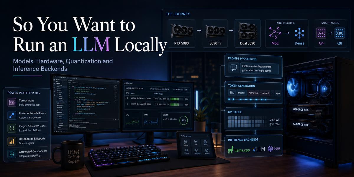
My own local LLM journey
My own setup is a practical example of why the model, hardware and backend should evolve around the workload rather than around specification sheets.
I did not begin with a carefully designed dual-GPU inference server. I arrived there through several iterations, each one exposing a different bottleneck.
Starting with an RTX 5080 and an MoE model
I started with an NVIDIA RTX 5080 with 16 GB of VRAM, running Qwen 3.6 35B-A3B.
This is a Mixture-of-Experts model. Although the model contains approximately 35 billion total parameters, only a much smaller subset is active for each generated token.
That made it an attractive starting point:
- It delivered strong capabilities for its active parameter count.
- Token generation was relatively fast.
- It fitted onto a modern consumer GPU.
- It was good enough to handle serious development tasks.
- It offered a low-friction introduction to local inference.
For many workloads, that combination would already be excellent.
However, after using it for repository-level development, I started to prefer the consistency of a dense model.
My typical tasks are not isolated code-completion exercises. They often involve reading several related files, following a multi-step implementation plan, understanding existing conventions and modifying components across a larger solution.
For that workload, predictable behaviour mattered more to me than the computational efficiency of the MoE architecture.
That led me to Qwen 3.6 27B.
Moving to an RTX 3090 Ti and a dense 27B model
My next setup used an RTX 3090 Ti with 24 GB of VRAM and Qwen 3.6 27B Q4.
Unlike the previous model, Qwen 3.6 27B is dense. All of its parameters participate in processing each token.
The Q4 quantisation allowed the model to fit onto a single 24 GB card while leaving enough space for the runtime and a useful KV cache.
This combination was already extremely capable.
It worked particularly well for:
- Multi-file code changes.
- C# Dataverse plugins.
- TypeScript and React applications.
- FetchXML and SQL.
- Power Automate and Logic Apps definitions.
- Azure DevOps pipelines.
- Repository-wide refactoring.
- Long implementation instructions.
The dense model produced the more consistent coding behaviour I was looking for.
Q4 was not a temporary or unusable compromise. It was genuinely good, and for most local developers it would be a sensible place to stop.
But I wanted to see how far the same model could go with less aggressive weight quantisation.
The next target was Q8.
Adding a second RTX 3090
A 27-billion-parameter Q8 model requires approximately 27 GB just for its quantised weights.
Once runtime buffers, CUDA overhead, vision components and the KV cache are included, it cannot fit properly on a single 24 GB GPU.
CPU offloading was technically possible, but that would reduce the responsiveness that made the local coding workflow valuable in the first place.
Instead, I added a second GPU:
- One RTX 3090 Ti with 24 GB of VRAM.
- One RTX 3090 with 24 GB of VRAM.
Together, the system provides 48 GB of aggregate VRAM.
Using vLLM with tensor parallelism, the model is distributed across both cards:
RTX 3090 Ti, 24 GB
          +
RTX 3090, 24 GB
          │
          ▼
48 GB aggregate VRAM
          │
          ▼
Qwen 3.6 27B Q8
The cards do not become one physically unified 48 GB GPU. Each card still owns its own memory, and the devices must communicate while performing inference.
However, tensor parallelism allows the model and its runtime state to be divided between both devices while remaining entirely in GPU memory.
My current configuration
The current setup runs:
- Qwen 3.6 27B dense model
- Q8 weight quantisation
- Q8 KV cache
- Up to a 262K-token context window
- Vision input
- vLLM serving
- Tensor parallelism across two GPUs
- 48 GB of aggregate VRAM
- An OpenAI-compatible API
This has become my main local coding model.
The journey also changed how I think about GPU selection.
The RTX 5080 is a newer GPU and substantially faster in many conventional workloads. However, its 16 GB of VRAM placed a hard limit on model size, quantisation and context capacity.
The RTX 3090 generation is older, less power-efficient and considerably warmer, but each card provides 24 GB of VRAM. For local inference, those additional gigabytes can be more valuable than a newer architecture.
The most important lesson was simple:
For local LLMs, memory capacity frequently determines what is possible. Compute performance determines how quickly you can do it.
Parameter count is only the beginning
Model names frequently include values such as 7B, 14B, 32B or 70B.
The “B” means billions of parameters.
A dense 32B model contains approximately 32 billion learned parameters, and all of its transformer layers participate in processing each token.
As a broad rule, larger models can represent more knowledge and more complex behaviour, but size alone does not determine quality. Training data, architecture, post-training, reasoning strategy and domain specialisation can matter just as much.
Dense models
In a dense model, essentially all model parameters are used for each generated token.
Dense models are comparatively straightforward to reason about:
- Total parameter count approximates the active parameter count.
- Weight memory grows directly with model size.
- Compute requirements grow broadly with model size.
Mixture-of-Experts models
Mixture-of-Experts, or MoE, models contain several expert subnetworks but activate only a subset for each token.
A model might contain 100 billion total parameters while activating only 10 billion or 20 billion for a particular token.
This can reduce computation relative to an equally large dense model, but there is an important trap:
Inference memory is influenced by the total parameters that must be loaded, not only the parameters activated for one token.
An MoE model can therefore be computationally fast while still requiring a large amount of VRAM or unified memory.
When evaluating an MoE model, check both:
- Total parameters, which strongly affect model storage and memory.
- Active parameters, which strongly affect compute per token.
My own move from Qwen 3.6 35B-A3B to Qwen 3.6 27B was not based on the assumption that dense models are universally better.
It was a workload-specific decision.
The MoE model was efficient and fast. The dense model gave me the consistency I preferred for complex repository work. Another workload, especially one prioritising throughput, might reach the opposite conclusion.
Understanding quantisation
Most open-weight models are originally distributed using 16-bit floating-point weights, commonly FP16 or BF16.
At 16 bits, every parameter requires approximately two bytes.
The raw weight memory can therefore be estimated as:
Weight memory ≈ parameters × bits per parameter ÷ 8
For example:
8B model at 16-bit   ≈ 16 GB
8B model at 8-bit    ≈ 8 GB
8B model at 4-bit    ≈ 4 GB

32B model at 16-bit  ≈ 64 GB
32B model at 8-bit   ≈ 32 GB
32B model at 4-bit   ≈ 16 GB

70B model at 16-bit  ≈ 140 GB
70B model at 8-bit   ≈ 70 GB
70B model at 4-bit   ≈ 35 GB
These figures cover only the raw weights. The runtime also needs memory for the KV cache, temporary buffers, model metadata, activations and the inference engine itself.
Quantisation compresses model weights into lower-precision representations. llama.cpp supports a broad range of integer quantisations, including 1.5, 2, 3, 4, 5, 6 and 8-bit formats, while vLLM supports formats including FP8, INT8, INT4, GPTQ, AWQ, GGUF, compressed tensors and hardware-specific schemes.
A practical quantisation guide
The exact result varies by model and quantisation method, but the following is a useful starting point.
| Format | Typical use |
|---|---|
| FP16 / BF16 | Maximum fidelity, training, fine-tuning and data-centre inference |
| FP8 | High-throughput inference on supported modern accelerators |
| Q8 / INT8 | High fidelity with approximately half the weight memory of FP16 |
| Q6 | Strong quality with moderate compression |
| Q5 | Quality-focused local inference |
| Q4 | Common balance between memory, speed and quality |
| Q3 | Running a larger model under a tight memory budget |
| Q2 and below | Experiments and severe memory constraints |
A good starting point for local inference is usually a modern 4-bit or 5-bit quantisation.
Moving from Q4 to Q8 doubles the weight memory, but it does not necessarily double answer quality.
In my own case, Qwen 3.6 27B Q4 was already a strong coding model. Moving to Q8 was an incremental quality decision rather than a transformation from unusable to usable.
The cost of that increment was significant:
Q4 weights
    │
    └── Fit on one 24 GB GPU

Q8 weights
    │
    └── Required two 24 GB GPUs plus tensor parallelism
That is a useful reminder that quantisation decisions cannot be separated from hardware decisions.
Conversely, moving from Q4 to Q2 may allow a much larger model to fit, but the additional parameters do not always compensate for aggressive precision loss.
The correct choice should be established through evaluation rather than folklore.
llama.cpp recommends quantising from a high-quality 16 or 32-bit source rather than requantising an already compressed model, because repeated quantisation can cause additional quality degradation.
GGUF, GPTQ, AWQ and Safetensors
Quantisation names are often mixed with model file formats and runtime formats, creating a small alphabet soup.
GGUF
GGUF is closely associated with llama.cpp and its ecosystem.
A GGUF file can include:
- Quantised model tensors.
- Model metadata.
- Tokeniser information.
- Chat-template information.
- Architecture details.
GGUF is particularly useful when you need:
- llama.cpp compatibility.
- CPU inference.
- Partial GPU offloading.
- Broad hardware support.
- Many quantisation choices.
- A single portable model file.
Safetensors
Safetensors is commonly used for Hugging Face and PyTorch model weights.
vLLM and SGLang typically consume Hugging Face model repositories containing Safetensors weights and configuration files.
These deployments often use:
- BF16 or FP16.
- FP8.
- AWQ.
- GPTQ.
- BitsAndBytes.
- Model-specific compressed-tensor formats.
GPTQ and AWQ
GPTQ and AWQ are weight-only quantisation approaches frequently used for GPU inference.
They can deliver good compression and performance, but backend and hardware compatibility must be checked before selecting a model. vLLM maintains a compatibility matrix because not every quantisation kernel is available on every accelerator generation.
The file that fits is not automatically the file that runs efficiently.
VRAM determines what fits
For GPU inference, VRAM is the first hard boundary.
Compute performance matters, but a fast GPU cannot efficiently run a model whose weights and cache do not fit.
A practical local guide looks roughly like this:
| Available accelerator memory | Realistic starting point |
|---|---|
| 6 to 8 GB | Small 3B to 8B models at 4-bit |
| 10 to 12 GB | 7B to 14B models at 4-bit |
| 16 GB | 14B models comfortably, some 20B to 27B models with tighter settings |
| 24 GB | 20B to 32B models at 4-bit, smaller models at higher precision |
| 32 GB | 32B-class models comfortably, larger models with aggressive quantisation |
| 48 GB | 27B models at Q8 with large cache budgets, or 70B-class models around 4-bit |
| 64 to 96 GB | 70B models with more context or precision, and some larger MoE models |
| 128 GB and above | Large dense and MoE deployments, depending on architecture |
These are planning estimates, not guarantees.
The actual requirement depends on:
- Quantisation format.
- Context length.
- KV cache precision.
- Number of concurrent sequences.
- Model architecture.
- Vision components.
- Backend overhead.
- Speculative decoding configuration.
My own 48 GB configuration prioritises a high-quality Q8 27B model, vision and a very large context window rather than using the same memory pool for a more aggressively quantised 70B model.
That is another example of workload-based selection.
A larger model is not always the better choice when it leaves too little memory for the context, cache or modalities the application actually needs.
The KV cache: the memory you did not budget for
During inference, the model stores attention keys and values from previously processed tokens.
This is the KV cache.
Without it, the model would need to recompute the entire conversation every time it generated another token.
The KV cache grows with:
- Context length.
- Number of transformer layers.
- Attention dimensions.
- Cache precision.
- Number of active users or sequences.
This is why a model may load successfully at a 4,096-token context and run out of memory at 64,000 tokens.
The advertised context window is not free storage hidden somewhere inside the model.
A simplified relationship is:
KV memory ∝ tokens × layers × KV dimensions × cache precision × sequences
Many modern models use grouped-query or multi-query attention to reduce KV-cache requirements, but long contexts and concurrency can still consume many gigabytes.
Some runtimes support quantised KV caches, trading a small amount of quality or compute overhead for significantly reduced memory use. vLLM supports quantised KV-cache configurations, while llama.cpp also exposes lower-precision cache types.
My current system uses a Q8 KV cache.
This provides a useful compromise:
- A much smaller cache than BF16.
- Higher precision than more aggressive FP8 or lower-bit cache configurations.
- Enough memory efficiency to expose a context window of up to 262K tokens.
- More space for large coding sessions, tool definitions and repository context.
That does not mean every request should contain 262,000 tokens.
Long context still increases prompt-processing time and consumes substantial cache memory. The important difference is that the capacity is available when a project genuinely requires it.
When sizing hardware, reserve memory for the actual context and concurrency you intend to use.
Do not calculate only the model file size and declare victory.
There are two different speeds
LLM benchmarks often report one number: tokens per second.
That number is incomplete.
Inference has two important phases:
- Prompt processing, also called prefill.
- Token generation, also called decode.
They behave very differently.
Prompt processing
Prompt processing reads and processes the input tokens before the first response token can be generated.
This includes:
- The system prompt.
- Conversation history.
- Retrieved documents.
- Tool definitions.
- Images or multimodal inputs.
- The latest user message.
Prompt processing can handle many input tokens in parallel, making it heavily influenced by compute throughput, memory movement, attention kernels and batching.
It is commonly measured as:
Prompt-processing tokens per second
Long prompts can produce impressive prompt-processing throughput while still creating a noticeable delay before the first generated token.
The user experiences that delay as time to first token.
A model might process a 10,000-token prompt at 1,500 tokens per second, requiring several seconds before generation even begins.
This becomes particularly important for coding assistants.
A development tool may submit:
- The current file.
- Several related source files.
- Repository instructions.
- Tool definitions.
- Conversation history.
- Build output.
- A diff.
- Documentation.
- The user's latest request.
The local model may generate only a few hundred response tokens, but it must first process tens of thousands of input tokens.
For that reason, prompt-processing performance can matter more than decode speed in repository-heavy workflows.
Token generation
Once the prompt has been processed, the model generates the response one token at a time.
Each new token depends on the previous token.
This makes decoding fundamentally sequential for a single request.
For many local, single-user workloads, token generation is strongly constrained by memory bandwidth because the model weights must be read repeatedly while each token is produced.
A useful theoretical approximation is:
Maximum decode tokens/s ≈ memory bandwidth ÷ model working-set size
Imagine a quantised model with a 16 GB working set running on hardware with 1,000 GB/s of memory bandwidth:
1,000 GB/s ÷ 16 GB ≈ 62.5 tokens/s
That is an optimistic ceiling.
Real performance will be lower because of:
- KV-cache access.
- Kernel overhead.
- Synchronisation.
- Quantisation and dequantisation.
- Memory inefficiency.
- Sampling.
- Backend overhead.
- Model architecture.
- Communication between GPUs.
This formula explains something that surprises many newcomers:
A GPU with substantially more compute is not automatically proportionally faster at single-user token generation.
Memory bandwidth and model size can matter more.
It also explains why dual-GPU inference does not automatically double generation speed.
Splitting the model across two cards solves a capacity problem, but tensor-parallel communication becomes part of every inference step. Depending on the hardware topology and backend, the result may offer slightly higher speed, similar speed or even lower single-request speed than a model contained on one sufficiently large GPU.
Capacity and speed are different axes.
Prompt caching changes the equation
Many enterprise requests share a large common prefix.
Examples include:
- The same system instructions.
- The same tool definitions.
- The same policy document.
- The same retrieved knowledge.
- Repeated questions about one long document.
- Multiple branches of an agent workflow.
- Repeated development requests against one repository.
Prefix caching stores the already computed KV cache for that shared prefix so it can be reused.
vLLM's automatic prefix caching allows requests with identical prefixes to skip the repeated computation of those tokens. SGLang uses RadixAttention to organise and reuse common prefixes efficiently.
Caching can dramatically improve time to first token when prompts contain large repeated sections.
It does not normally make the actual generation of new output tokens faster.
That distinction matters:
- Prefix caching improves repeated prompt processing.
- Speculative decoding targets token generation.
For coding workloads, prompt caching is particularly valuable when the tool repeatedly includes stable repository instructions, tool definitions or shared project context.
Speculative decoding
Speculative decoding uses a faster draft mechanism to predict several future tokens.
The main model then verifies those tokens in a batch.
The technique works because checking several proposed tokens together can be more efficient than generating them sequentially with the full model.
llama.cpp supports several speculative-decoding approaches, including a separate draft model and model-specific draft mechanisms. vLLM also supports multiple speculative strategies.
The speed-up depends on:
- Draft-model speed.
- Token acceptance rate.
- Target-model architecture.
- Batch size.
- Prompt and output characteristics.
- Additional memory use.
A poor draft model may generate many rejected tokens and add complexity without improving performance.
As usual, benchmark the actual workload.
Choosing hardware
Local inference can run on CPUs, consumer GPUs, workstation accelerators, Apple Silicon and data-centre hardware.
Each option solves a different problem.
CPU-only inference
CPU inference has the lowest barrier to entry.
llama.cpp supports x86, ARM, Apple Silicon and other processor architectures, and can run quantised models without a discrete GPU.
CPU inference is useful for:
- Learning.
- Small models.
- Background classification.
- Embeddings.
- Low-frequency automation.
- Systems without a supported GPU.
- Partial model offloading.
Its primary limitation is memory bandwidth.
Modern desktop CPUs may have considerable compute capability, but system RAM is much slower than high-end GPU memory. Token generation for medium and large models can therefore feel glacial, even when the model technically fits.
CPU inference is often viable for a small number of tokens or asynchronous workloads. It is less attractive for interactive use with larger models.
NVIDIA consumer GPUs
NVIDIA currently offers the broadest path through the local LLM software garden.
CUDA support is well established across llama.cpp, vLLM, SGLang, PyTorch, Transformers and most specialised inference kernels.
Typical consumer options include:
- 8 to 16 GB cards for small and medium models.
- 24 GB cards such as the RTX 3090 and RTX 4090.
- 32 GB cards such as the RTX 5090.
A used RTX 3090 remains particularly interesting for local AI because it offers 24 GB of memory and mature CUDA support.
My own journey illustrates the trade-off clearly:
RTX 5080
16 GB VRAM
Newer architecture
Fast compute
Limited model capacity

RTX 3090 Ti
24 GB VRAM
Older architecture
More model capacity

RTX 3090 Ti + RTX 3090
48 GB aggregate VRAM
Enough for Qwen 3.6 27B Q8,
vision and a large Q8 KV cache
Two 24 GB cards can host models that do not fit on one card, although combining GPUs introduces additional complexity:
- Sufficient power delivery.
- Case airflow.
- Physical slot spacing.
- PCIe lane allocation.
- NUMA and CPU considerations.
- Backend-specific multi-GPU behaviour.
- Increased idle and load power.
- More failure points.
- Communication overhead between devices.
llama.cpp can split model layers or tensors across multiple GPUs, while vLLM supports tensor, pipeline, data, expert and context parallelism for distributed inference.
Multi-GPU capacity does not automatically scale single-user performance linearly. Communication between devices can become part of every token.
AMD GPUs
AMD hardware can be attractive when it offers more memory or better pricing, but the software path must be checked carefully.
vLLM supports AMD GPUs and several AMD-compatible quantisation paths, while llama.cpp can use HIP and Vulkan backends. Compatibility remains dependent on the particular accelerator, operating system, kernel and quantisation method.
For an experienced Linux operator, AMD can be a viable option.
For somebody looking for the broadest range of copy-and-paste installation instructions, NVIDIA remains the path with fewer thorns.
Apple Silicon
Apple Silicon uses unified memory shared by the CPU and GPU.
This allows a Mac with 64, 128, 256 or even 512 GB of unified memory to load models that would require several discrete GPUs elsewhere.
Apple's MLX-LM project supports text generation, quantisation and LoRA fine-tuning on Apple Silicon. llama.cpp also treats Apple Silicon as a first-class platform with Metal acceleration.
Apple Silicon is attractive when you value:
- Large unified-memory capacity.
- Low noise.
- Power efficiency.
- Simple desktop operation.
- Running very large quantised models on one machine.
It is less ideal when you require:
- CUDA-only software.
- NVIDIA-specific quantisation kernels.
- Maximum production-serving throughput.
- Easily replaceable or upgradeable GPUs.
- Broad Linux data-centre tooling.
A Mac can be a formidable personal inference workstation, but it is not merely an NVIDIA server with a fruit logo.
Data-centre GPUs
Data-centre accelerators provide features that consumer GPUs may not:
- Larger VRAM pools.
- ECC memory.
- Enterprise support.
- High-speed GPU interconnects.
- Better virtualisation options.
- Rack-oriented cooling.
- Predictable availability.
- Hardware support for formats such as FP8.
They are the appropriate choice when local AI becomes a shared platform rather than one person's workstation.
At that point, hardware selection should be driven by:
- Required model precision.
- Concurrent users.
- Requests per second.
- Context distribution.
- Availability targets.
- Power and cooling.
- Cluster topology.
- Support contract.
- Total cost of ownership.
The local AI barrier to entry
There is no single barrier to local AI. There are several gates.
Level 1: “I want to try a model”
Requirements:
- An existing Windows, macOS or Linux computer.
- LM Studio or Ollama.
- A small quantised model.
- No coding required.
This is the easiest entry point.
LM Studio provides a desktop interface for finding, downloading and running local models. It can also expose OpenAI-compatible and Anthropic-compatible APIs. Its llmster daemon supports headless operation without the desktop GUI.
Ollama provides a compact command-line workflow and partial OpenAI API compatibility, making it easy to connect existing applications to a locally managed model.
Level 2: “I want to build an application”
Requirements:
- A stable local API.
- A defined model version.
- Authentication or network isolation.
- Prompt templates.
- Error handling.
- Basic monitoring.
- Repeatable startup configuration.
At this stage, LM Studio, Ollama or llama.cpp can all work well.
Level 3: “Several people need to use it”
Requirements:
- Concurrency.
- Continuous batching.
- Capacity management.
- Request queues.
- Rate limits.
- Health checks.
- Logging.
- Containerisation.
- Model lifecycle management.
This is where vLLM and SGLang become increasingly attractive.
Level 4: “This is a production service”
Requirements:
- Redundancy.
- Multiple inference workers.
- Load balancing.
- Metrics and tracing.
- Automated deployment.
- Security reviews.
- Versioned model artefacts.
- Regression evaluations.
- Rollback procedures.
- Capacity and failure testing.
At this stage, the model is only one component of the platform.
The barrier to running a model is now low.
The barrier to running one reliably remains considerably higher.
Choosing an inference backend
The backend is the software engine that loads the model, manages memory, schedules requests and exposes an API.
Selecting the right backend can matter as much as selecting the GPU.
llama.cpp
llama.cpp is a lightweight C and C++ inference project designed to run models across a very broad range of hardware.
Its server currently supports:
- CPU and GPU inference.
- GGUF quantisations.
- OpenAI-compatible chat, completions and Responses endpoints.
- Anthropic-compatible messages.
- Embeddings.
- Reranking.
- Structured JSON output.
- Function calling.
- Parallel decoding.
- Continuous batching.
- Multimodal input.
- Speculative decoding.
- Multi-user operation.
Choose llama.cpp when:
- You use GGUF models.
- You need CPU inference.
- You want partial CPU and GPU offloading.
- You have unusual or mixed hardware.
- You want maximum quantisation flexibility.
- You are serving one or a few users.
- You want one portable binary and a simple server.
- You need to fit the largest possible model into limited memory.
Think twice when:
- You need very high concurrent throughput.
- You are operating a large homogeneous GPU cluster.
- You rely heavily on Hugging Face-native model formats.
- You need the newest specialised CUDA kernels immediately.
- You want enterprise-scale scheduling across many workers.
llama.cpp has grown far beyond a command-line toy. Its server now includes continuous batching and parallel request handling, but its greatest strength remains flexibility rather than operating a warehouse full of GPUs.
I used llama.cpp during the single-GPU phase of my own setup because it provided excellent GGUF support, flexible quantisation and granular control over context and cache settings.
It is particularly good when the main question is:
How can I make this model fit efficiently on the hardware I already own?
vLLM
vLLM is designed primarily for efficient model serving.
Its architecture focuses on throughput, concurrency and memory-efficient scheduling.
Important capabilities include:
- PagedAttention for KV-cache management.
- Continuous batching.
- Chunked prefill.
- Prefix caching.
- Distributed inference.
- Tensor, pipeline, data, expert and context parallelism.
- OpenAI-compatible APIs.
- Anthropic Messages compatibility.
- gRPC.
- Structured outputs.
- Tool and reasoning parsers.
- LoRA serving.
- Many quantisation formats.
- NVIDIA, AMD and CPU support.
PagedAttention divides KV-cache memory into blocks rather than requiring one large contiguous allocation for every sequence. This reduces memory fragmentation and helps the engine serve requests with different context lengths efficiently.
Chunked prefill divides long prompts into smaller chunks and schedules them alongside decode requests. In vLLM V1, chunked prefill is enabled by default where supported, prioritising active decode requests before scheduling additional prefill work.
Choose vLLM when:
- Several users or applications share the model.
- Throughput matters more than minimal setup.
- You use Hugging Face model repositories.
- You need tensor parallelism across GPUs.
- You want efficient dynamic batching.
- You need production-oriented serving.
- You need structured output or tool-call parsers.
- You are building an internal OpenAI-compatible endpoint.
Think twice when:
- Your model exists only as an unusual GGUF quant.
- You need extensive CPU offloading.
- You run primarily on Apple Silicon.
- You are using unsupported model architectures.
- You want a simple desktop application.
vLLM is usually the more natural option when the question changes from “How fast can one user generate?” to “How many requests can this server handle?”
In my case, vLLM also became necessary when I moved from one GPU to two.
Tensor parallelism allows Qwen 3.6 27B Q8 to be distributed across both 24 GB cards, while vLLM manages the KV cache, long context, vision input and OpenAI-compatible serving layer.
The backend therefore did not change merely because I wanted a different API.
It changed because the hardware topology and serving requirements changed.
SGLang
SGLang is another high-performance serving framework for language and multimodal models.
It is designed for low latency and high throughput from a single GPU to distributed clusters. Its runtime includes RadixAttention for prefix reuse, structured output, speculative decoding, parallelism and specialised scheduling.
RadixAttention organises cached prompt prefixes in a tree-like structure. This is particularly useful when many requests share components such as system prompts, retrieved documents or agent instructions.
Choose SGLang when:
- Prefix reuse is central to the workload.
- You are building complex agent or reasoning systems.
- You need aggressive serving optimisation.
- You operate modern GPU infrastructure.
- You are comfortable tuning a more specialised runtime.
- Structured and constrained generation are important.
- You want to benchmark beyond the standard vLLM path.
Think twice when:
- You are beginning with local AI.
- You want a desktop-friendly workflow.
- The deployment has only one occasional user.
- Operational simplicity matters more than squeezing out additional throughput.
SGLang is a powerful engine, but it is not normally the first rung of the ladder.
Ollama
Ollama focuses on model management and accessibility.
It provides:
- Simple model download and execution.
- A local API.
- OpenAI API compatibility.
- Integrations with developer tools.
- GPU acceleration across several platforms.
Choose Ollama when:
- You want the fastest path from zero to a local API.
- You value simple model packaging.
- You are prototyping integrations.
- You are building a developer workstation.
- You do not need deep control over every runtime parameter.
Think twice when:
- You need maximum throughput.
- You need precise control over batching and cache allocation.
- You operate a large multi-GPU service.
- You need a specialised quantisation or kernel configuration.
Ollama is an excellent front door. It does not have to be the entire building.
LM Studio and llmster
LM Studio combines a polished desktop interface with developer APIs.
It supports:
- Model discovery and download.
- Local chat.
- Model loading and unloading.
- OpenAI-compatible endpoints.
- Anthropic-compatible endpoints.
- Native REST and language SDKs.
- API-token authentication.
- Headless server operation through
llmster.
Choose LM Studio when:
- You are learning local AI.
- You need to compare models interactively.
- You want a GUI and an API in one tool.
- You want a simple local development server.
- You later want to move the same workflow to a headless Linux server.
LM Studio has evolved beyond “a GUI for chatting with GGUF files.” Its headless daemon makes it viable for lab servers and small internal deployments, although high-concurrency production serving remains a different operational category.
MLX-LM
MLX-LM is designed for running and fine-tuning language models on Apple Silicon.
It supports:
- Hugging Face model integration.
- Text generation.
- Quantisation.
- LoRA and QLoRA fine-tuning.
- Prompt caching.
- An API server.
Choose MLX-LM when:
- Apple Silicon is your primary platform.
- You want native access to unified memory.
- You need efficient experimentation or fine-tuning on a Mac.
- You prefer Python and Hugging Face-style workflows.
For Apple hardware, MLX-LM should be evaluated alongside llama.cpp rather than assuming that every model must be converted to GGUF.
Backend comparison
| Backend | Best fit | Model ecosystem | Hardware flexibility | Concurrency | Entry difficulty |
|---|---|---|---|---|---|
| LM Studio | Desktop exploration and small APIs | GGUF and supported local formats | High | Low to moderate | Very low |
| Ollama | Simple local model management | Ollama model packages | High | Low to moderate | Very low |
| llama.cpp | Portable, quantised local inference | GGUF | Very high | Moderate | Low to moderate |
| MLX-LM | Apple Silicon | Hugging Face / MLX | Apple-focused | Moderate | Low to moderate |
| vLLM | Production GPU serving | Hugging Face / Safetensors | High on supported platforms | High | Moderate |
| SGLang | Optimised agentic and prefix-heavy serving | Hugging Face / Safetensors | Modern accelerators | High | Moderate to high |
There is no universal winner.
A sensible progression is:
LM Studio or Ollama
        ↓
llama.cpp
        ↓
vLLM or SGLang
        ↓
Clustered production platform
Do not begin with Kubernetes, three inference engines and a distributed cache because you want to ask a 7B model where it left the semicolon.
A practical hardware selection path
Existing laptop or desktop
Start with:
- LM Studio or Ollama.
- A small 4-bit instruct model.
- A context between 4K and 16K.
- One user.
- A simple evaluation set.
Do not buy anything yet.
GPU with 8 to 12 GB
Target:
- 3B to 8B models.
- Some 12B to 14B models with 4-bit quantisation.
- Short or medium contexts.
- One interactive user.
This can be enough for classification, extraction, writing assistance and lightweight coding.
GPU with 16 GB
Target:
- 7B to 14B models comfortably.
- Some 20B-class or efficient MoE models at low precision.
- Vision models with controlled context.
- Local development and individual assistants.
My RTX 5080 and Qwen 3.6 35B-A3B configuration occupied this category. The model's MoE architecture made it possible to obtain strong performance despite the limited VRAM.
GPU with 24 GB
Target:
- 20B to 32B models at approximately 4-bit.
- Smaller models at Q8 or FP8 where supported.
- Longer contexts with careful KV-cache settings.
- Small-team inference.
- Experimentation with speculative decoding.
This is currently one of the most useful local AI memory tiers.
My RTX 3090 Ti and Qwen 3.6 27B Q4 setup demonstrated why. It provided enough memory for a capable dense model, a useful context and fully GPU-resident inference.
GPU with 32 GB
Target:
- 32B models with more breathing room.
- High-quality quantisations.
- More KV-cache capacity.
- Better concurrency.
- Larger multimodal models.
- Some 70B experiments with aggressive compression or offloading.
Two 24 GB GPUs
Target:
- Dense 27B to 32B models at Q8.
- 70B-class models around 4-bit.
- Large KV-cache budgets.
- Vision models.
- Tensor or model splitting.
- Higher aggregate concurrency.
- Production experiments.
Budget for the rest of the machine:
- A suitable motherboard.
- Sufficient PCIe slots.
- A large power supply.
- Serious cooling.
- Adequate system RAM.
- Physical space.
- Noise.
Two discounted GPUs can quietly assemble a very expensive radiator.
Large Apple unified-memory system
Target:
- Large quantised models on one device.
- Personal research.
- Long-context experimentation.
- Quiet workstation operation.
- Models that exceed consumer GPU VRAM.
Prioritise memory capacity first, then memory bandwidth.
Enterprise server
Target:
- Multiple users.
- High availability.
- vLLM or SGLang.
- Observability.
- Automated deployment.
- Load testing.
- Redundant nodes.
- Security and governance.
At this point, begin with service-level objectives, not a shopping cart.
Using a local LLM for Power Platform development
Power Platform projects are unusually good candidates for a capable local coding model because they are often both context-heavy and token-heavy.
A real project may combine:
- C# Dataverse plugins.
- JavaScript or TypeScript web resources.
- Power Apps code apps.
- Power Automate cloud flows.
- Logic Apps workflows.
- FetchXML.
- SQL 4 CDS queries.
- Dataverse table and column metadata.
- Solution component definitions.
- Azure DevOps pipelines.
- Deployment documentation.
- Error traces.
- Existing architectural decisions.
These components rarely live in isolation.
A change to a Dataverse table may require updates to a plugin, a flow, a Code App, a query and the deployment pipeline. A coding assistant that sees only the active file is working through a keyhole.
Connecting the local model to Visual Studio Code
My vLLM server exposes an OpenAI-compatible endpoint.
I connect that endpoint to Visual Studio Code through the GitHub Copilot Chat model workflow, allowing the local Qwen model to participate directly in repository-level development.
The architecture looks roughly like this:
Power Platform repository
          │
          ▼
Visual Studio Code
          │
          ▼
GitHub Copilot Chat interface
          │
          ▼
OpenAI-compatible vLLM endpoint
          │
          ▼
Qwen 3.6 27B Q8
This gives the local model access to the development context selected by the editor and coding agent.
The large context window is particularly useful here.
A single development request can include:
- Repository instructions.
- Current and related files.
- Existing code patterns.
- Tool definitions.
- Build errors.
- Test output.
- Previous implementation steps.
- Dataverse metadata.
- Documentation.
- A long conversation history.
The 262K context capacity does not mean every request should be that large. It means I do not need to begin each task by aggressively removing context that may become important later.
Abundant local implementation tokens
The implementation phase of software development consumes a large number of tokens.
The model repeatedly needs to:
- Read files.
- Search the repository.
- Generate code.
- Review errors.
- Inspect build output.
- Apply corrections.
- Re-read modified files.
- Produce explanations.
- Iterate until the project works.
Paying a frontier model to process every one of those intermediate steps can become expensive, particularly across larger Power Platform repositories.
A local model changes the economics.
Once the hardware exists, the marginal cost of another implementation iteration is primarily electricity and time rather than metered API tokens.
This makes it practical to let the coding agent inspect more context, attempt more iterations and work through large tasks without watching a token counter tick like a taxi meter.
A hybrid planner, worker and reviewer architecture
The most effective workflow I found was not replacing frontier models entirely.
It was assigning different models to different roles.
Frontier model
Plans and decomposes the work
          │
          ▼
Local Qwen 3.6 27B Q8
Implements the tasks
          │
          ▼
Frontier model
Reviews the result
The frontier model acts as the architect.
It receives the broader requirement, reasons about the solution and produces a structured implementation plan.
The local model acts as the developer.
It works inside the repository, reads the relevant files, writes the code, runs tools, handles errors and completes the token-intensive implementation.
The frontier model then acts as the reviewer.
It examines the result, compares it with the original requirements and identifies architectural, security or logical issues that may have been missed.
The model roles resemble a familiar engineering process:
Architect → Developer → Reviewer
This pattern is particularly effective for Power Platform work.
The frontier model can reason about architecture across Dataverse, Azure, Power Apps and integration boundaries. The local model can then perform the verbose implementation work: editing plugins, flows, pipelines, configuration files and frontend components.
Finally, the frontier model reviews the complete change rather than paying to participate in every intermediate edit.
Approximately 90% fewer frontier-model tokens
For suitable development tasks, this workflow has reduced my frontier-model token consumption by approximately 90%.
That number is based on my own workflow rather than a universal benchmark. The actual saving depends on:
- The size of the repository.
- The complexity of the task.
- How independently the local model can work.
- How much context the frontier model needs.
- The number of review cycles.
- Whether escalation is required.
The saving is possible because implementation usually consumes far more tokens than planning and review.
Instead of using the most expensive model for every repository search, file edit and error correction, I reserve it for the stages where its additional reasoning capability creates the most value.
The local model handles the high-volume middle.
This does not eliminate quality controls. The final review remains part of the process.
The objective is not:
Make the local model do everything.
It is:
Use frontier intelligence where it has the highest impact, and use abundant local tokens for the implementation work.
For my Power Platform projects, that hybrid architecture has provided the best balance of quality, context capacity, privacy and cost.
Benchmark the workload you actually have
A useful benchmark should separate:
- Short-prompt prefill.
- Long-prompt prefill.
- Short response generation.
- Long response generation.
- Single-user latency.
- Multi-user throughput.
- Cold model start.
- Warm model performance.
- Cached-prefix performance.
- Maximum stable context.
For example:
pp512       Process a 512-token prompt
pp8192      Process an 8,192-token prompt
tg128       Generate 128 tokens
tg512       Generate 512 tokens
c1          One concurrent request
c8          Eight concurrent requests
Also record:
- Time to first token.
- End-to-end latency.
- Tokens per second per request.
- Total server throughput.
- Peak VRAM.
- GPU power.
- Queue time.
- Error rate.
For a coding workload, also consider testing:
repo-small      5K to 10K input tokens
repo-medium     25K to 50K input tokens
repo-large      100K or more input tokens
tool-loop       Multiple model and tool iterations
vision          Screenshot or architecture-diagram analysis
A server generating 300 tokens per second in aggregate may still feel slow if each of twenty users receives only 15 tokens per second after waiting in a queue.
Similarly, a model with excellent decode performance may feel slow inside Visual Studio Code if every request starts with a 100,000-token prompt that is processed inefficiently.
Throughput and user experience are related, but they are not twins.
What should you choose?
For a developer testing local models:
Start with LM Studio or Ollama.
For a single workstation using quantised models:
Use llama.cpp, LM Studio or Ollama.
For Apple Silicon:
Evaluate both MLX-LM and llama.cpp.
For a shared Linux GPU server:
Start with vLLM.
For agent-heavy workloads with repeated prefixes and aggressive performance requirements:
Benchmark SGLang against vLLM.
For unusual hardware, mixed CPU/GPU inference or extreme quantisation:
Start with llama.cpp.
For a large local coding model distributed across NVIDIA GPUs:
Evaluate vLLM with tensor parallelism.
For production:
Benchmark at least two backends using your model, prompts, context distribution and expected concurrency.
The real optimisation hierarchy
Local LLM optimisation often becomes a hunt for command-line flags.
The order of impact is usually much simpler:
1. Choose the right task and model
2. Ensure the model fits fully in fast memory
3. Select an appropriate quantisation
4. Use the right backend
5. Configure context and KV cache
6. Enable prefix caching
7. Tune batching and concurrency
8. Evaluate speculative decoding
9. Adjust low-level kernel parameters
My own hardware journey followed almost exactly that path.
I first changed the model architecture, moving from MoE to dense.
Then I changed the GPU to gain more memory.
Then I changed the quantisation from Q4 to Q8.
That required adding another GPU.
Finally, I changed the backend to vLLM because the model now required tensor parallelism, a larger KV cache, vision support and a standard API for development tools.
No scheduler flag could have made the 27B Q8 model fit into 16 GB.
No amount of additional VRAM would have made the MoE model behave exactly like the dense model I wanted.
And no benchmark would have mattered if the final system did not perform well inside my actual Power Platform development workflow.
Final recommendation
Local AI has become genuinely accessible.
A developer can install a desktop application, download a quantised model and expose a compatible API in minutes. llama.cpp can run across an enormous variety of hardware. Apple systems can load models using large pools of unified memory. vLLM and SGLang can turn GPU servers into high-throughput inference platforms.
But accessibility should not be confused with simplicity.
A useful local LLM system requires alignment between:
- The task.
- The model.
- The quantisation.
- The context window.
- The hardware.
- The backend.
- The concurrency model.
- The operational environment.
Start small.
Measure prompt processing and token generation separately.
Buy memory before chasing theoretical compute.
Treat context as a memory budget.
Choose llama.cpp for flexibility, vLLM for production throughput and multi-GPU serving, SGLang for advanced serving, LM Studio or Ollama for accessibility, and MLX-LM for Apple-native workflows.
Most importantly, benchmark your own prompts.
My own setup grew from a single RTX 5080 running an efficient MoE model into a dual-GPU, 48 GB vLLM server running Qwen 3.6 27B at Q8, with a Q8 KV cache, vision support and a context window of up to 262K tokens.
That system now handles the token-intensive implementation work inside Visual Studio Code, particularly for large Power Platform projects.
A frontier model plans the work and reviews the result. The local model performs the implementation.
For tasks that fit this workflow, it has reduced my frontier-model token consumption by approximately 90% without a noticeable reduction in the quality of the final reviewed result.
Local inference did not replace the cloud.
It gave me a much better place to spend the tokens.
The local AI ecosystem is moving too quickly for one permanent answer, but the engineering questions remain refreshingly stable:
Does it fit?
Is it fast enough?
Is it accurate enough?
Can we operate it reliably?
Everything else is configuration.